Intro to Forecasting Lifetime Value for Mobile Apps

What is LTV?

LTV, or the Lifetime Value of a user, is a powerfully informative metric whose purpose is to give decision makers an idea as to what a new user’s monetary worth is. Moreover, when produced from a forecasting model, LTV can be calculated for some point in the future, using current data. In simplest form, LTV is calculated as the monetary contribution that an average user will generate during their lifespan.

Because LTV is such a popular topic it’s not surprising that the internet is a cornucopia of links to different LTV models, examples, and discussions. Yet, how you apply any of these models will vary depending on the intended use and your company’s business model.

In general, the approach to calculating LTV includes two major inputs; retention and revenue. A third input that may be added is a referral or virality factor, to account for the number of additional new users each new user may refer.

When it comes to modeling LTV, there are a couple of generalized approaches one can take.

The first is using regression and curve fitting. Regression modeling in general is very popular and can uncover the relationships between variables of interest and their drivers of impact (stand by for our series of posts on regression analysis!). The benefit of this approach is that it is flexible and can be applied to several different data points for retention, revenue, and virality. Taking the time to understand the non-linear forms of regression, like polynomial regression, can also help to build accurate models when the data isn’t nice and linear.

The second, and most accurate, approach to modeling LTV is the probabilistic approach. Probabilistic models can be challenging to create, as they require a deeper understanding of statistics, specifically the nuances between the different probability distributions (e.g. the poison, exponential, and gamma distribution). In the probabilistic approach, the type of relationship the business has with its users (i.e. contractual or non-contractual) is combined with the data type used (i.e. discrete or continuous), and from there the appropriate model may be selected. The benefit of probabilistic models is that they can investigate engagement behavior on an individual user level and thus create a consumer-lifetime-value (CLV) model which can be aggregated into an LTV model.

Unlike regression models, probabilistic models do not try to identify and measure the countless factors that motivate a user’s behavior. Instead, they focus on the probability of the desired outcome. We will share our experience and learnings in handling this sense of randomness in future posts.

 

Formulating the LTV model.

The method we’ll focus on in this post is the regression-based approach first introduced to me by Eric Seufert’s presentation, “Two Methods for Modeling LTV with a spreadsheet”. Here he breaks down LTV into two components:

- Lifetime = Retention
- Value = Monetization

He then uses the regression approach to predict lifetime, and refers to it as the “Retention Approach” where LTV is calculated in the following manner:

LTV = ARPDAU * User-Days

With ARPDAU being average revenue per daily active user and, “user-days” being the number of days the average user will be active at the time we wish to forecast for.

Using simulated ARPDAU data (average revenue per daily active user), we ask ourselves the question: For users acquired from a specific time frame and segment, what will their lifetime value be at some date in the future, such as 21 or 30 days after install?

We begin by collecting retention data from a specific user segment, and then tabulate the data into cohort format. From this data set we calculate the retention rate for every day after the initial date of install, as well as the ARPDAU for each day after the initial install. We then create a retention curve using the power function and use that model to calculate the forecasted retention input for our LTV formula.

 

The Retention Curve:

It would be great if the trendline in all our retention graphs remained a flat, horizontal line, but unfortunately such a phenomenon defies reality. When a new user downloads an app and starts to use it, they will inevitably ask themselves whether they want to continue using the app or not. When a user chooses the latter and stops engaging, we no longer consider them a “live’ user, but rather a “dead” user. In this sense, our retention curves are very similar to a survival curve, where with each passing day, the number of users that are alive start to dwindle away. Remember this iconic line from Fight Club: “On a long enough timeline, the survival rate of everyone drops to zero.” If I had to guess, this is what Eric meant when he said that the retention curve is essentially a survival curve, and why his model assumes that the retention curve follows a power function; it’s the same idea.

 

Building the Model:

As mentioned previously, we constructed our retention curve by calculating the retention rate for each day after install. Then, based on the assumption that the power function (y = a * x^b) will best describe the retention data and with “days-after-install” for all available “x”s, and “retention rate” for all available “y”s, we estimated the parameters a and b using the following functions in Excel:

- “a” = EXP(INDEX(LINEST(LN(all available x’s),LN(all available y’s)),2))
- “b” = INDEX(LINEST(LN(all available x’s),LN(all available y’s)),1)

Using all of our historical data points available, we can estimate the parameters “a” and “b,” giving us the model:

y = 0.6 * (x)^-0.4, where x = the days after install we wish to forecast for.

The output of the model gives us the predicted retention rate, and the area below the retention curve is the user-days. To calculate this value, we sum all the forecasted retention rates between day 1 and the day we wish to forecast for. This range of values is known as the integral.

 

Visualizing the model:

In this post, we won’t dive too deep into the subject of R squared, but it is one commonly used way of assessing how well a model fits the data. To start, we used all available data and plotted both the actual and the predicted retention rates. Then, using Excel’s trend-line function we found that the power function has an R-squared of 98.33%, as seen in graph 1. This indicates that less than two percent of the variation is not explained by our model. But what happens when we don’t use all available data, and how will that impact the models accuracy?

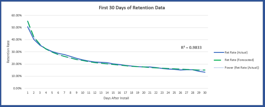
Graph 1 - user retention curve

To investigate how the model’s accuracy changes with less data, we trained the model with two different intervals of historic retention data and then use that model to forecast user-days at different points in the future.

As shown in graph 2, we started by training the model using the first 7 days of retention data, then forecasted the number of user-days we would have at 14, 21, and 30 days after install.

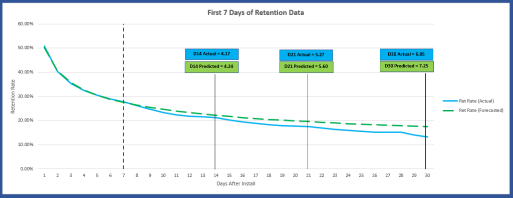
Graph 2. - predicted user retention curve

As you can see, there is little difference variance between the actual and predicted user-days when using the first 7 days of historic data. What’s important to note here is that the value we’re using in our LTV equation is the number of user-days (the integral for the forecast period) and not the retention rate itself.

Next, we used 14 days of data to train the model and forecast user-days for 21 and 30 days after install, as seen in graph 3.

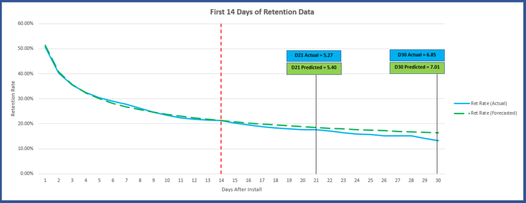
Graph 3. Trained, predicted user retention curve

Training the model with an additional seven more days of data did result in a smaller difference between the actual and predicted values for both the 21 and 30-day forecasts.
Using $0.15 as the simulated trailing ARPDAU data, and our LTV equation (LTV = ARPDAU * User-Days), we can make the same comparison but in terms of LTV, as shown in table 1.

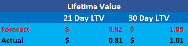
Table 1. - 21 and 30-day user LTV forecast

When we look at the difference between the forecasted and actual LTV values, we can see that the gap between the forecast and actual is smaller with the 21-day forecast than it is with the 30-day forecast. This highlights a commonly known limitation to forecasting which is; your short-term forecasts will be more accurate than your long-term forecasts. There are several reasons for this is the case and we’ll cover them in future posts. For now, just keep in mind that the further out your forecasts are, the less accurate they’re going to be.

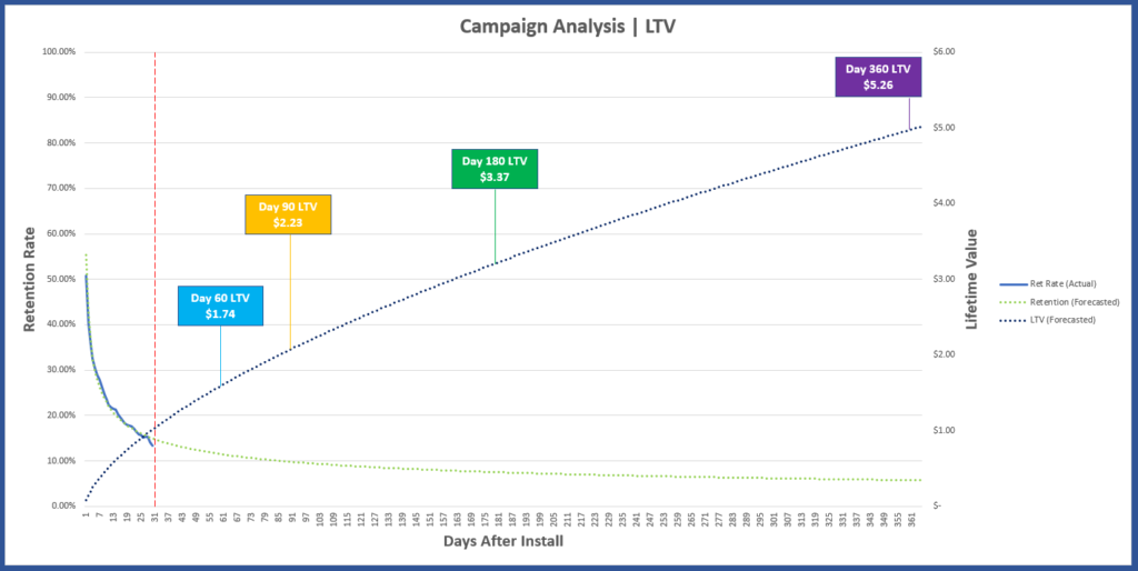
Graph 4. - User LTV forecast

Using all available retention data to train our model, and our LTV equation, we create an LTV curve and make forecasts for; 60, 90, 180, and 360 days after install (graph 4). As tempting as it might be to marvel in our ability to create a crystal ball from a spread sheet and make all sorts of decisions based on our predictions; we should keep in mind that this basic model assumes ARPDAU ($0.15) is constant.

Once more, forecasts generally lose their accuracy the further out we try to make them. Keeping this does of reality in mind can help ensure we don't make decisions based on less accurate data firstly, but more importantly it serves to motivate us to continue exploring for ways to make predictive analytics more accurate over longer terms. While there are additional methods that can help improve the accuracy of the ARPDAU input over the longer term, we assumed a constant ARPDAU of $.15 simply as part of today's introduction to LTV.

In our next post we’re going to dive into another application of the regression approach to modeling LTV, where we use historical average revenue per user (ARPU) data to make lifetime value forecasts.

 

Conclusions:

With this post we wanted to help readers who have little or no prior experience with predictive analytics, by providing a basic and functional approach to forecasting LTV. For anyone who wants to take a deeper dive into this type of predictive analysis, a few topics worth exploring are:

- Regression validation.
- Time series.
- Sample Size (“How much data should I use?”).

There are other, slightly more sophisticated methods to create a model for forecasting user-days, and we’re excited to cover the probabilistic approach to predicting a user’s lifespan cover in future posts. But for this analysis we found that this approach to predicting LTV was straightforward and could easily be created in a spreadsheet. This method also served as the main inspiration for our other explorations into LTV too, so with that said we highly recommend you try using this approach with some of your own data and reach out to us (hello@incipia.co) to share your experience with this method.

 

Be sure to bookmark our blog, sign up to our email newsletter for new post updates and reach out if you're interested in working with us to optimize your app's ASO or mobile marketing strategy.

Incipia is a mobile marketing consultancy that markets apps for companies, with a specialty in mobile advertising, business intelligence, and ASO. For post topics, feedback or business inquiries please contact us, or send an inquiry to projects@incipia.co